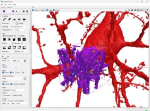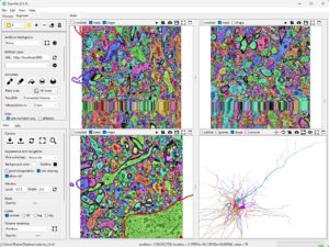


Below are some example Python scripts to generate volumes of regions within the released datasets of the fragment of the human cerebral cortex. The published article describing the data can be found here:
https://www.science.org/doi/10.1126/science.adk4858
The released dataset is listed here:
https://h01-release.storage.googleapis.com/data.html
The script below prints out the header information of the data.
# pip install numpy itk cloud-volume
import numpy as np
from cloudvolume import CloudVolume

# Uncomment to select which data you want information of:
vol = CloudVolume("gs://h01-release/data/20210601/4nm_raw", use_https=True)
# vol = CloudVolume("gs://h01-release/data/20210601/c3/", mip=0, use_https=True)
# vol = CloudVolume("gs://h01-release/data/20210601/masking", mip=0, use_https=True)
# vol = CloudVolume("gs://h01-release/data/20210601/c2/", mip=0, use_https=True)

# Retrieve the dimensions of the volume at the specified MIP level
volume_dimensions = vol.volume_size
print("Volume dimensions at MIP 0:", volume_dimensions)

# Data type
data_type = vol.dtype
print("Data type of the volume:", data_type)

# Number of channels (if applicable)
num_channels = vol.num_channels
print("Number of channels in the volume:", num_channels)

# Bounding box (if defined, provides info on the spatial extent of the data)
bounding_box = vol.bounds
print("Bounding box of the volume:", bounding_box)

# Scale and resolution info
for mip in range(len(vol.scales)):
    scale_info = vol.scales[mip]
    print(f"MIP {mip} info: resolution {scale_info['resolution']}, size {scale_info['size']}")
Now, use the Neuroglancer web-based viewer to select the center location of the slice or volume you want to save. This volume will be saved as a .nii file, which includes the correct voxel spacing and origin.
# pip install numpy itk cloud-volume
import numpy as np
from cloudvolume import CloudVolume
import matplotlib.pyplot as plt
import itk

# Use the neuroglancer-demo to select a location
location_at_8nm = [247489, 193590, 2002]

# Uncomment this for a small cubic volume
# image_size = 512
# z_size = 512

# Uncomment this for a larger center plane
image_size = 512*8
z_size = 1

# Select the level of detail
mip_level = 3

# Have a look at the resolutions at the various mip levels above to understand this:
location_at_mip_level = [location[0]/4, location[1]/4, location[2]]

vol = CloudVolume("gs://h01-release/data/20210601/4nm_raw", mip=mip_level, progress=False, use_https=True, fill_missing=True)

resolution = vol.scales[mip]['resolution']

cutout = vol[location_at_mip_level[0]-np.floor(image_size/2):location_at_mip_level[0]+np.ceil(image_size/2), location_at_mip_level[1]-np.floor(image_size/2):location_at_mip_level[1]+np.ceil(image_size/2), location_at_mip_level[2]-np.floor(z_size/2):location_at_mip_level[2]+np.ceil(z_size/2)]

cutout = np.transpose(cutout)
cutout = np.array(cutout)

# Uncomment to visualise the center slice
# plt.imshow(cutout[0,(int)(z_size/2),:,:])

# Convert the NumPy array to an ITK image
image_itk = itk.image_from_array(cutout[0,:,:])

# Set the voxel spacing
spacing = (resolution[0], resolution[1], resolution[2])  # Spacing for each dimension
image_itk.SetSpacing(spacing)

# Set the origin
origin = ((location_at_mip_level[0]-(image_size/2))*resolution[0], (location_at_mip_level[1]-(image_size/2))*resolution[1], (location_at_mip_level[2]-(z_size/2))*resolution[2])  # Origin for each dimension
image_itk.SetOrigin(origin)

# Save the image to a file in NIFTI format
itk.imwrite(image_itk, 'image.nii')

print("Done")
The same can be done for the label map with a few modifications since this data is stored with a different level of detail compared to the raw imaging data.
# pip install numpy itk cloud-volume
import numpy as np
from cloudvolume import CloudVolume
import matplotlib.pyplot as plt
import itk

# Use the neuroglancer-demo to select a location
location_at_8nm = [247489, 193590, 2002]

mip_level = 2

# Uncomment this for a small cubic volume
# image_size = 512
# z_size = 512

# Uncomment this for a larger center plane
image_size = 512*8
z_size = 1

# Have a look at the resolutions at the various mip levels above to understand this:
location_at_mip_level = [location[0]/4, location[1]/4, location[2]]

vol = CloudVolume("gs://h01-release/data/20210601/c2/", mip=mip_level, progress=False, use_https=True, fill_missing=True)

resolution = vol.scales[mip]['resolution']

# Define the region of the image based on the location, image_size and z_size.
cutout = vol[location_at_mip_level[0]-np.floor(image_size/2):location_at_mip_level[0]+np.ceil(image_size/2), location_at_mip_level[1]-np.floor(image_size/2):location_at_mip_level[1]+np.ceil(image_size/2), location_at_mip_level[2]-np.floor(z_size/2):location_at_mip_level[2]+np.ceil(z_size/2)]

# Reduce the precision since ScanXm can only load 255 labels anyway.
cutout = cutout.astype(np.uint16)
cutout = np.transpose(cutout)
cutout = np.array(cutout)

# Uncomment to visualise the center slice
# plt.imshow(cutout[0,(int)(z_size/2),:,:])

# Convert the NumPy array to an ITK image
image_itk = itk.image_from_array(cutout[0,:,:])

# Set the voxel spacing
spacing = (resolution[0], resolution[1], resolution[2])  # Spacing for each dimension
image_itk.SetSpacing(spacing)

# Set the origin
origin = ((location_at_mip_level[0]-(image_size/2))*resolution[0], (location_at_mip_level[1]-(image_size/2))*resolution[1], (location_at_mip_level[2]-(z_size/2))*resolution[2])  # Origin for each dimension
image_itk.SetOrigin(origin)

# Save the image to a file in NIFTI format
itk.imwrite(image_itk, 'c2.nii')

print("Done")
The same works for the mask that identifies neuropil, nuclei, blood vessels, myelin, and fissures.
# pip install numpy itk cloud-volume
import numpy as np
from cloudvolume import CloudVolume
import matplotlib.pyplot as plt
import itk

# Use the neuroglancer-demo to select a location
location_at_8nm = [247489, 193590, 2002]

mip_level = 0

# Uncomment this for a small cubic volume
image_size = 512/2
z_size = 512/2

# Uncomment this for a larger plane
# image_size = 512*4
# z_size = 1

# Have a look at the resolutions at the various mip levels above to understand this:
location_at_mip_level = [location[0]/8, location[1]/8, location[2]/2]

vol = CloudVolume("gs://h01-release/data/20210601/masking", mip=mip_level, progress=False, use_https=True, fill_missing=True)

resolution = vol.scales[mip]['resolution']

# Define the region of the image based on the location, image_size and z_size.
cutout = vol[location_at_mip_level[0]-np.floor(image_size/2):location_at_mip_level[0]+np.ceil(image_size/2), location_at_mip_level[1]-np.floor(image_size/2):location_at_mip_level[1]+np.ceil(image_size/2), location_at_mip_level[2]-np.floor(z_size/2):location_at_mip_level[2]+np.ceil(z_size/2)]

# Reduce the precision since ScanXm can only load 255 labels anyway.
cutout = cutout.astype(np.uint16)
cutout = np.transpose(cutout)
cutout = np.array(cutout)

# Uncomment to visualise the center slice
# plt.imshow(cutout[0,(int)(z_size/2),:,:])

# Convert the NumPy array to an ITK image
image_itk = itk.image_from_array(cutout[0,:,:])

# Set the voxel spacing
spacing = (resolution[0], resolution[1], resolution[2])  # Spacing for each dimension
image_itk.SetSpacing(spacing)
# Set the origin
origin = ((location_at_mip_level[0]-(image_size/2))*resolution[0], (location_at_mip_level[1]-(image_size/2))*resolution[1], (location_at_mip_level[2]-(z_size/2))*resolution[2])  # Origin for each dimension
image_itk.SetOrigin(origin)

# Save the image to a file in NIFTI format
itk.imwrite(image_itk, 'mask.nii')

print("Done")
Now, use the Neuroglancer viewer again to select the neurons and get their IDs. These can then be used to download the surface mesh as a .ply file, which can be loaded into ScanXm and will automatically be in the same reference space as the imaging data.
from cloudvolume import CloudVolume
import trimesh

vol = CloudVolume('gs://h01-release/data/20210601/c3', use_https=True)

# Select the mesh from the neuroglancer-demo
mesh = vol.mesh.get(4897964007, lod=0)
#mesh = vol.mesh.get(5057903946, lod=0)
#mesh = vol.mesh.get(4796545315, lod=0)
#mesh = vol.mesh.get(5203884133, lod=0)
#mesh = vol.mesh.get(4926903194, lod=0)
#mesh = vol.mesh.get(5261382769, lod=0)

vertices = list(mesh.values())[0].vertices
faces = list(mesh.values())[0].faces

# Instantiate Trimesh
mesh_trimesh = trimesh.Trimesh(vertices=vertices, faces=faces)

# Save mesh
mesh_trimesh.export('mesh.ply')

print("Done")
